Economic Order Quantity (EOQ): what it is, formula, and how to calculate

How much idle capital do you have in your warehouse right now? And how many times have you run out of stock of your fastest-moving product?

Most businesses purchase inventory based on past orders or intuition: they order a large batch because "shipping was cheaper," or small, constant orders because "that way it doesn't accumulate." 

Unfortunately, these types of decisions are not usually reflected in the short term or on an invoice, but rather in capital tied up in slow-moving inventory, in the warehouses needed for extra inventory. 

The good news is: there's a formula over 100 years old that solves exactly this question. It's called EOQ (Economic Order Quantity) and in this guide, we show you what it is, how to calculate it step-by-step, and, most importantly, how much money you can save by applying it, with a real "before and after" case study.

What is the EOQ Model (Economic Order Quantity)?

The EOQ (Economic Order Quantity) is the exact quantity of units you should order in each purchase order to ensure your total inventory costs are as low as possible.

Simply put: it answers the question "How much should I order each time?" with a calculated number.

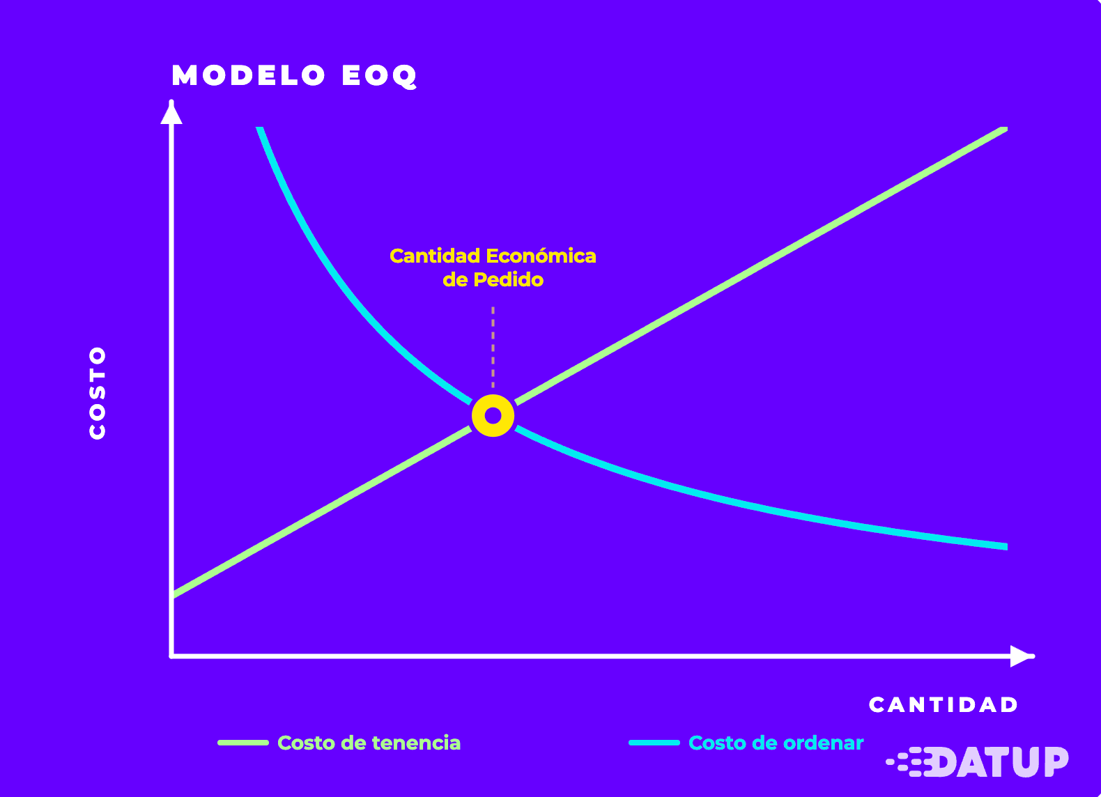
The model starts from a tension that every business owner knows, even if they haven't named it. There are two forces pulling in opposite directions:

• Ordering small and often: less capital tied up and lower storage costs, but you pay the cost of placing orders many, many times a year (transport, administration, receiving).
• Ordering a lot at once: you save on ordering costs, but you fill your warehouse with merchandise that takes months to sell, tying up cash and paying for storage.

The EOQ finds the exact equilibrium point between these two lines of reasoning: the lot size where the sum of both costs reaches its minimum.

EOQ defined in one sentence: the EOQ is the order quantity that minimizes the sum of ordering cost plus inventory holding cost. Not so much that capital gets tied up in the warehouse, nor so little that you're constantly placing purchase orders.

What is it for and why is it crucial in logistics?

These are the benefits of calculating the EOQ and ordering inventory based on it:

• You reduce your total inventory cost. The EOQ doesn't just minimize storage or just orders: it minimizes the sum of both. It is the only mathematically optimal point in your entire purchasing policy.
• You free up trapped cash flow. By no longer buying giant batches "just in case," you recover capital that was dead on the shelves. That money returns to your operations.
• You simplify the purchasing decision. No more asking "how much should I order this time?". You have a clear rule: when it's time to restock, you order approximately your EOQ.
• You better plan your cash flow and warehouse. With a standard lot size, you know how much capital you'll tie up and how much warehouse space you'll need throughout the year.

Ultimately, EOQ transforms a decision typically made out of habit ('we've always ordered this way') into a data-driven decision. And in supply chain, data trumps narrative.

Advantages and Disadvantages of the EOQ System

No model is perfect, and being honest about its limitations is part of using it well.

Model Limitations or Assumptions

The classic EOQ operates within an idealized world. In practice, you need to understand its assumptions to know when to adjust it:

1. It assumes constant and known demand. The model assumes you sell at a stable and predictable rate throughout the year. If your product has strong seasonality or peaks due to promotions, this assumption weakens.
2. It does not consider volume discounts. In its basic version, EOQ ignores that your supplier might offer you a better price per unit if you buy more. Sometimes it's worth ordering more than the EOQ just for the discount.
3. It assumes constant costs and instantaneous replenishment. It does not explicitly incorporate variable lead times, capacity constraints, or real-world supply issues.

That's why EOQ is an excellent benchmark. It gives you the optimal number in a stable world; your business judgment adjusts it to the reality of your operation.

The EOQ Formula Explained

Here's the core of the model. Don't be intimidated by the square root: behind it are just three variables you already know from your business.

EOQ = √ (2 × D × S) / H

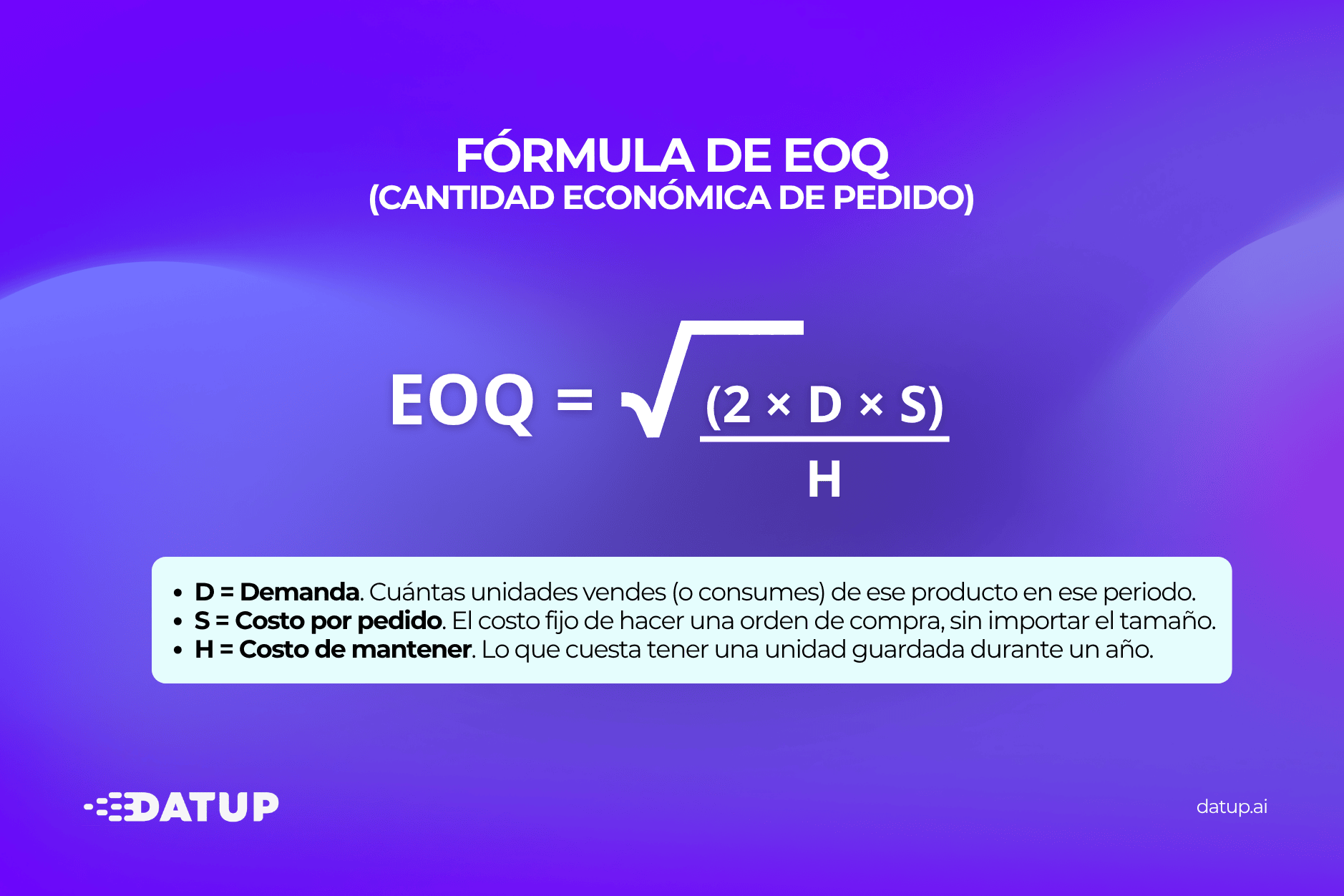
Where each acronym stands for:

D: Annual Demand

It's the simplest: the total number of units of that SKU you move in a year. If your store sells 10,000 pairs of a shoe model per year, then D = 10,000.

S: Cost per Order (Setup cost)

It's what it costs you each time you generate a purchase order, regardless of whether you order 100 or 1,000 units. That's why it's considered a "fixed cost per order." This includes:

• Administrative costs: your team's time generating the order, recording the invoice, reconciling the payment.
• Order Logistics: transportation from the supplier to your warehouse, handling, and receiving of goods.
• Management: document issuance, supplier coordination, quality inspection upon receipt.

H: Inventory Holding Cost (Holding cost)

It's the cost of holding a unit in storage for one year. It's almost always the most underestimated cost, because a good portion of it is invisible:

• Storage: warehouse rent, shelving, utilities, security.
• Personnel: the salaries of those who manage, count, and move that inventory.
• Insurance and Depreciation: insurance against theft or damage, physical deterioration, obsolescence.
• Financial Cost of Capital: the money invested in that merchandise that you can't use for anything else. This opportunity cost is real, even if it doesn't come as an invoice.

At the EOQ point, the total ordering cost and the total holding cost end up being practically equal. When those two figures balance out, you've found your optimal lot size.

Practical example of using EOQ

Theory is all well and good, but the true value of EOQ becomes clear when you apply it to real money. 

A shoe store that sells a best-selling model, the "UrbanSport" sneakers. Here are its annual figures:

Before calculating the EOQ, let's see what happens when the owner orders haphazardly. For this, we'll use two simple formulas:

• Annual ordering cost: (D ÷ Q) × S → number of orders times the cost per order.
• Annual holding cost: (Q ÷ 2) × H → the average inventory (half the lot size) times its unit cost.

Where Q is the lot size she chooses. Let's look at the two most common mistakes.

Scenario without EOQ (high costs from arbitrary purchasing)

Error A: "I order everything once a year" (Q = 10,000)

She buys all 10,000 pairs in one single giant order to save on shipping costs.

• Number of orders: 10,000 ÷ 10,000 = 1 order
• Ordering cost: 1 × $50 = $50
• Average inventory: 10,000 ÷ 2 = 5,000 pairs sitting in storage
• Holding cost: 5,000 × $2 = $10,000
• Total cost: $50 + $10,000 = $10,050

Almost no ordering cost, but an exorbitant storage cost: it has an average of 5,000 pairs tying up cash all year.

Error B: "Small, frequent orders" (Q = 100)

To avoid accumulation, it places small orders of 100 pairs.

• Number of orders: 10,000 ÷ 100 = 100 orders per year
• Ordering cost: 100 × $50 = $5,000
• Average inventory: 100 ÷ 2 = 50 pairs
• Holding cost: 50 × $2 = $100
• Total cost: $5,000 + $100 = $5,100

‍

The problem here is the opposite: it incurs almost no storage cost, but it places purchase orders 100 times a year, driving up the ordering cost.

What both cases demonstrate: neither the giant lot ($10,050) nor the micro-orders ($5,100) are efficient. Both are far from optimal.

Applying the EOQ Model (calculation and demonstrated savings)

Now let the formula decide. We apply the EOQ step-by-step:

EOQ = √ (2 × 10,000 × 50) / 2

1. Multiply the numerator: 2 × 10,000 × 50 = 1,000,000
2. Divide by H: 1,000,000 ÷ 2 = 500,000
3. Take the square root: √500,000 ≈ 707 pairs

The optimal order quantity is 707 pairs per order. Let's see how much this policy costs:

• Number of orders: 10,000 ÷ 707 ≈ 14.1 orders per year
• Ordering cost: 14.1 × $50 ≈ $707
• Average inventory: 707 ÷ 2 ≈ 354 pairs
• Holding cost: 354 × $2 ≈ $707
• Total cost: $707 + $707 ≈ $1,414

Notice the detail we mentioned earlier: the ordering cost ($707) and the holding cost ($707) ended up practically identical. That's the hallmark of the optimal point.

Comparative Savings

Let's put the three scenarios side by side:

• Savings versus the giant batch (A): $10,050 − $1,414 = $8,636 annually
• Savings versus micro-orders (B): $5,100 − $1,414 = $3,686 annually

Read that again: just by adjusting how much is ordered in each order, without selling an extra pair or changing suppliers, the store frees up between $3,686 and $8,636 annually. That's money that was hidden in a poor batch decision.

Variations and Extensions of the Economic Order Quantity Model

The classic EOQ is the foundation, but the reality of your operation sometimes requires more comprehensive models. These are the most common:

• EOQ with volume discounts: adjusts the calculation when the supplier offers a better unit price beyond certain quantity thresholds. Sometimes it's beneficial to order more than the pure EOQ just to capture the discount.
• EOQ with planned shortages (backorders): considers cases where you accept temporary, controlled stockouts, balancing the cost of the shortage against that of holding inventory.
• Multi-product models: when multiple SKUs share a budget, warehouse space, or transport capacity, and you need to optimize the whole, not each product in isolation.

The point is this: the EOQ is the first building block, not the whole house. Once you master the optimal lot size for one SKU, scaling it to hundreds or thousands of products with variable demand is another story.

The "sawtooth" graph and its relationship with ROP

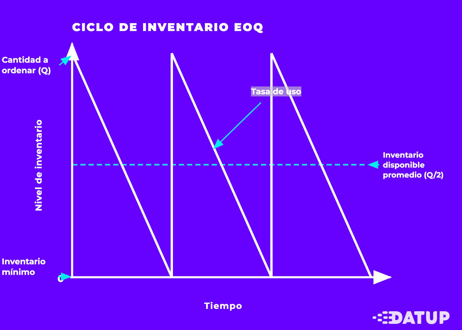
If you visualize your inventory over time under an EOQ policy, you'll see a pattern called "sawtooth": a series of triangles that go down and then back up.

It works like this:

• The horizontal axis is time; the vertical axis is your stock level.
• The line drops as you sell, at a rate tied to your demand.
• When inventory reaches the reorder point (ROP), you place an order for your EOQ quantity.
• After the lead time, the order arrives and inventory jumps back up. The cycle repeats.

Here's the question that confuses almost everyone: how do EOQ and ROP differ? They are two pieces of the same puzzle, but they answer different questions:

Working with both is what gives you a robust inventory policy: the EOQ tells you how much and the ROP tells you when. If you want to delve deeper into the second, we have a complete guide on how to calculate the reorder point (ROP).

Optimize your inventory today

EOQ is one of those tools that, with a pen, paper, and your business numbers, already starts saving you money. For a SKU, the calculation you saw above is sufficient and powerful.

But let's be honest about its limitations. Classic EOQ assumes constant demand, ignores seasonality, doesn't account for variable lead times or volume discounts. We know that calculating this manually in Excel, SKU by SKU, multiplies the risk of human error and becomes unmanageable when you have hundreds or thousands of products, each with its own demand, supplier, and behavior.

When you reach that point, it's no longer a formula problem: it's a problem of scale and up-to-date data.

At Datup , we dynamically calculate optimal order quantities by connecting directly to your ERP and WMS, and adjusting models with AI that learns your business: seasonality, real lead times, demand variability, and over 200 external variables like weather and inflation. Without external consultants and with results from the first few weeks.

Do you want to see how much capital you have tied up in inventory right now? Schedule a personalized demo with your own data and we'll show you the exact number, no obligation.

FAQs

Who created the EOQ model?

It was developed by Ford Whitman Harris, a Westinghouse production engineer, who first published the formula in 1913. It was one of the first scientific contributions to inventory management. Later, in 1934, consultant R. H. Wilson popularized it in industry and academia, making it a standard in industrial engineering.

What is the difference between EOQ and the Reorder Point (ROP)?

EOQ answers how much to order (the optimal lot size). ROP answers when to order (the inventory level that triggers a new order, considering lead time and safety stock). They are complementary: together they form a complete replenishment policy.

Is the EOQ model useful for service companies?

EOQ is designed for physical products that are stored, so it doesn't directly apply to pure services. However, it is useful for any service company that handles supplies or materials (a mechanic's workshop with spare parts, a clinic with medical supplies, a restaurant with non-perishable ingredients). As long as there's an ordering cost and a holding cost, EOQ has something to tell you.

How often should I recalculate my EOQ?

EOQ is not a number you calculate once and forget. It's advisable to review it when its variables change: if your demand goes up or down, if the supplier adjusts freight costs, or if warehousing and insurance costs increase. Recalculating it periodically keeps it a living tool, not a dead data point.